Rising Rate Suspension: A Design Guide

Understanding the influence of the mechanical leverage generated by the numerous linkages on a race car is critical.

The piston has leverage over the crankshaft proportional to the moment arm of the rod bearings, the aerodynamic centre of pressure finds its placement through the leverage that the rear wing has over the axles, the brake calliper has leverage over the wheel via the moment arm generated by the disc radius. A few examples of many.

Everyone is familiar with the concept of torque and mechanical advantage, The greater the radius of force application from the pivot point or fulcrum, the greater the leverage which is generated.

Since energy (work) output can never exceed the energy input, physics dictate that a force input at a large radius is multiplied by a smaller output radius and vice versa.

Understanding this concept with simple fulcrums and lever arms working in one plane is pretty elementary - the leverage of input vs. output has a linear relationship (check this article for more detail on linear levers):

Where 'F' is the force and 'L' indicates the respective radii.

Automotive suspension systems generate leverage during wheel displacement to actuate the spring-damper. With traditional wheel mounted spring-dampers (for example MacPherson struts) this leverage can often be approximated as linear throughout the wheel travel. This is fairly straightforward situation in which the spring rate increases approximately linearly with wheel displacement.

On the other side, more advanced configurations mount the spring-damper to the chassis, which offers a new dimension of design options and performance advantages to engineers.

In addition to the packaging advantages that come with these pushrod (or pullrod) actuated systems, reductions in unsprung weight and improved aerodynamic performance are also found. The challenge is in designing a linkage to translate the vertical motion of the wheel into linear motion of the spring-damper, which is often oriented out-of-plane to the wheel.

This introduces a device known as the bell crank - a component which changes the direction of forces by introducing a rotational pivot or fulcrum into the mechanism.

Suspension assembly of a F3 car highlighted featuring the pushrod, bell-crank (purple) and spring-damper

The bell crank also allows the magnitude of leverage generated by the system to be customised to the application at hand, but importantly for us it introduces non-linearity into the leverage, which will be the subject of the rest of this article.

Advantage Given

To understand the advantage to be had by utilising non-linearities, its first important to understand the fundamentals behind certain performance variables which must be respected in the design of an effective race car.

Firstly, i want to note that the majority of inboard systems are implemented on chassis’ which experience a relatively high amount of aerodynamic load. Thats a big clue.

As aerodynamic load increases with speed, the vertical force acting to compress the springs increases non-linearly. With a linear wheel rate (spring rate experienced at the wheels), the heave stiffness of the springs required to support the chassis at high speeds would simply destroy grip levels at lower speeds with the high contact patch load variations that would result.

Systems which offer a wheel rate that provides the aerodynamic support required at high speeds and the compliance required to generate sufficient mechanical grip at lower speeds would certainly carry a large benefit in these cases - increasing the width of the performance window in which a car is able to operate effectively.

The addition of a third, heave spring of course addresses this problem, but a platform incorporating a wheel rate which increases in magnitude with wheel displacement and produces a progressive, or rising leverage from the springs is another step forward.

Inboard suspension systems are often featured on high downforce cars such as this Oreca LMP1 chassis. This configuration also allows for rising rate geometry and a third, heave spring to be used.

Progressive rates would also have benefits in roll. The ability to implement a non-linear roll stiffness (and therefore non-linear roll gradient) has distinct advantages in that the aerodynamic platform would be kept in a more consistent range of the aeromap throughout different corner types (i.e. high speed, large radius and low speed, small radius).

Chart 1: A graph highligting the difference in leverage vs. ride height between non-linear suspension and linear configurations

Through varying the non-linearities at each axle, theoretically it can even open up the possibility of lateral acceleration dependant roll stiffness variation i.e. a varying chassis balance with speed.

So how do systems incorporating bell cranks achieve this kind of performance and how do you approach their design?

The Physics

The physics behind the relative forces and displacements generated by the bell crank introduce a little more maths, so lets approach them step by step and use a worked example to clearly understand the principles behind it.

Figure 1: An illustration of the worked example showing important variables

There are essentially two approaches to this:

1. Use a force based approach to characterise and tune the system's leverage based on the target wheel rates i.e. for ride height at Vmax.
   

2. Design the motion ratio around the target wheel travel and damper travel restrictions. The spring rate would then be defined accordingly.

I’ll cover both methods in the following section.

1. Use the Force:

The multiplication of force input to output, or the leverage ratio is mathematically fairly straightforward in principle and is linked to the relative size (radii) of the lever arms and the instantaneous angle of the lever arms respective to the direction of forces.

I’ll get straight into the analysis.

As we know, moment equilibrium must be reached in any static mechanical system, so we start with the understanding that:

The mechanical leverage of the spring over the wheel can then be defined as:

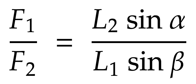
With the angles α and β known, this calculation is trivial.

In this case, which is the design condition at ride height, the spring force has an advantage of x1.718 over the wheel.

Observing how this leverage changes as ride height advances enables us to characterise a particular linkage and understand how the spring force is amplified in various dynamic situations.

By understanding how α and β evolve with ride height, we can start to put some numbers on it, but as these angles are changing relative to eachother depending on the design of the whole linkage the trigonometric relationships start to get a little complex, and so do the maths.

Life would be simple if we could simply use Pythagoras theorem, but as there are often no perfect right angle triangles in the real world, we have to apply the Cosine rule, which in a general sense is expressed as follows.

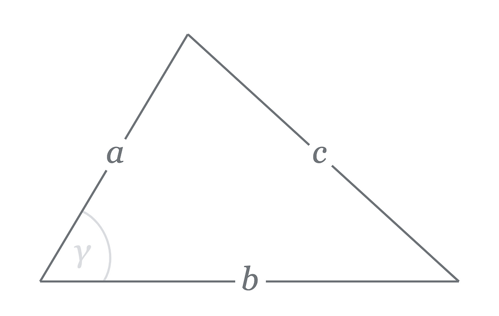
Let's construct our example bell crank based on the following inputs.

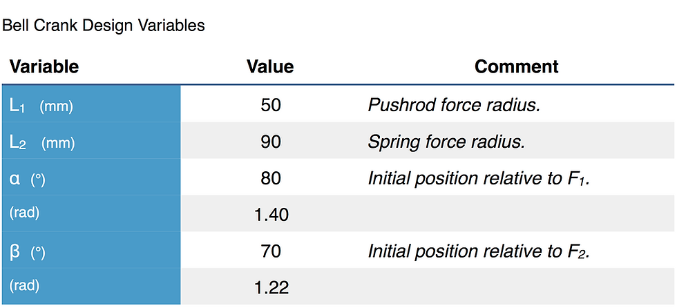
The length of the pushrod and damper are important here, so to complete the triangle, an imaginary line (d1) must be drawn between the pushrod mount at the wheel, to the pivot point of the bell crank. This allows us to calculate some important angles. (See Figure 1)

Unless you’re using a CAD package, finding the length of this line is the first application of the Cosine rule, adapted to use our variables:

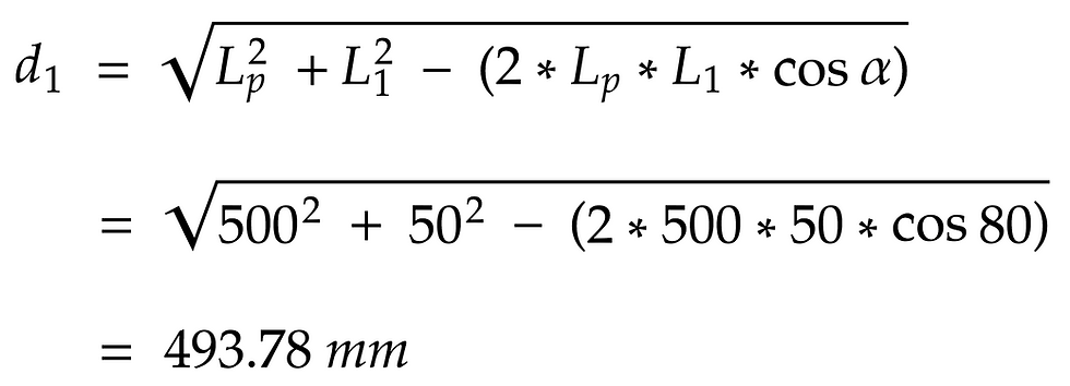
Similarly, the same technique is used for the other side of the bell crank. Damper length (Ld) in the design condition is known, so we find the length of an imaginary line linking the mounting point of the damper at the chassis to the pivot of the bell crank using the cosine rule again.

d1 and d2 remain constant throughout this study as they are between two static points

γ is an important angle here as it allows us to quantify the angular displacement of the bell crank due to any wheel travel.

So again in the design condition, we find γ using a rearranged version of the Cosine rule to identify the angle adjacent to α.

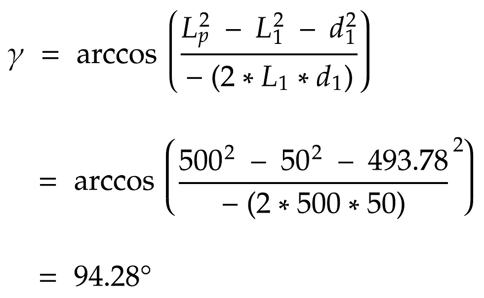
Disclaimer: I didn’t want this article to turn into a mess of maths, so throughout these calculations,the assumption is made that Lp simply extends in length as ride height changes which is of course not strictly true - its attachment point, being located on the upright is not static and therefore its position influences α and γ. Just bare this in mind if you’re using the method in your designs.

With that said, the next step is to calculate α in a displaced condition, let's say +25mm to represent 25mm of bump travel. This is calculated using the Cosine rule again, with Lp = 525.

α' is our new input for equation (1), which we'll use again a little later.

This also means γ' in the displaced condition (Lp = 525) is 126.41°

The bell crank rotation with this change in ride height is then γ' - γ = + 32.13°

Now as γ and θ share the same axis of rotation, we only need to subtract this this rotation from θ to calculate θ', which we’ll use to calculate β' as the second angular input into equation (1).

So in the design condition:

To find θ' :

With θ' known, Ld in the displaced condition can be found:

A 49.7mm displacement. This new dimension feeds into the following formula to find β':

So, wrapping that up, the leverage of the system over the wheel at this displacement as a proportion of the spring force is calculated by using the new values of α' and β' back into equation (1):

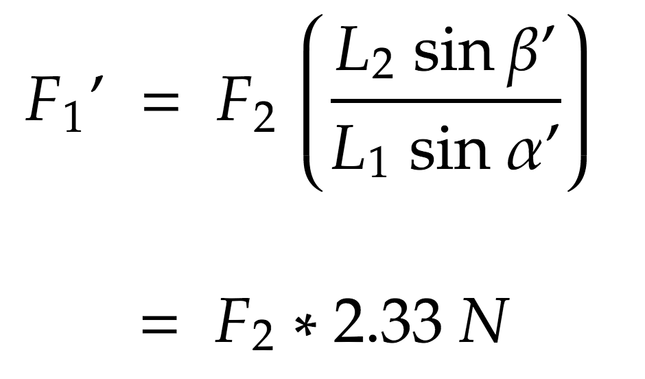
Yeah.. I was tired too! If you guys have a preferred way of doing this, please do comment and leave your thoughts. I always appreciate different approaches, this is just the one i arrived at.

Repeating this over the entire range of wheel travel - the following curve of leverage vs. angular displacement is produced.

Chart 2: Leverage vs. Ride height plotted for our worked example.

With a certain leverage ratio in mind, you can calculate α and β to give the desired advantage and work backwards to define the geometry.

2. Question of Displacement:

It may be important to your design that you understand the relationship between spring displacement and wheel travel, in which case you need to understand the motion ratio of the linkage.

The good news is that all the maths are already outlined above, so the same process applies - i won't repeat it here.

Mathematically, this is simply the ratio of damper movement relative to wheel movement over a particular displacement. For the system designed above over the same 25mm of compression travel:

Again, this can be plotted over the range of wheel travel to understand how it changes throughout the entire range of compression and bump travel.

Chart 3: Motion Ratio vs. Ride height plotted for our worked example.

As mentioned, this method is more appropriate if you have a target wheel travel and are using a specific damper with a set range of travel.

For example; knowing you have 80mm of damper travel and a design target of 50mm wheel travel allows you to set the motion ratio at 1.6 by designing bell crank input and output radii to produce the required deflections. You then set a spring rate to suit.

Subtract the Maths

So if you weren’t particularly interested in the maths, its enough to summarise the response of a system like this with respect to two main parameters:

• Lever length: The lever length, or the ratio of lever lengths is the important parameter in defining the force multiplication of the system and defining the motion ratio.

The relative proportion of these lengths is whats key. If the lever arm for the spring (L2) is longer than the lever arm for the pushrod (L1), the spring will see larger movement than the wheel and therefore the force produced by the spring will have an advantage over the wheel.

Lever lengths don’t define the gradient of the curve but do define the magnitude or gain of the curve.

• Lever angles: Lever angle relative to the direction of force input and output are the big players in defining the curve of these linkages.

Because we’re working with trigonometry and periodic functions, some interesting observations are made.

If the two angles sum to 180°, the leverages are equal to 1 and the rate is linear

If the angles sum to < 180°, the rate is progressive, likewise if they sum to > 180°, the rates are regressive.

These relationships hold true enough to be approximate in the typical range of design conditions most linkages will sit in, where the angle between the two arms is close to 90°.

As long as the above relationships are respected, it’s not difficult to get the behaviour you want.

With high aerodynamics loads and cornering forces, DTM is another championship suited to rising rate suspension.

Caution

Care must be taken to get the relative angles you’re designing into a bell crank set correctly - it’s not always an intuitive relationship to realise the point at which your leverage starts to behave unexpectedly.

If you’re not calculated with your design, you can inadvertently design a system which produces a regressive rate.

I once was told a story about an older BTCC car design in which the suspension geometry produced a regressive rate - once it had fallen below a certain bump travel, it didn’t get back up to ride height..! Surely an engineer's worst nightmare.

Closing out

That about wraps this one up.

This analysis has all been in 2D, if you’re working in 3D like some systems do, you’ve got another layer of complexity but the approach is still valid. The Cosine rule is very useful.

Of course if you have a CAD program available to you this all becomes relatively trivial, but as always it’s a great benefit to understand the mechanics behind what you’re doing to allow you to be efficient with your design and truly understand why it works.

This kind of non-linear leverage is also used in motorcycles and bicycles with rear suspension. It’s employed on linkages to create a progressive response which ensures the damper doesn’t bottom out on larger, high energy compression inputs.

Similarly to race cars, a weaker spring leverage at ride height is favourable for compliance and grip, but the added dimension of frequency response in these applications places extra emphasis on rider comfort, so the motivations for progressive systems are double.

Non-linear suspension designs feature in many applications, here's another one on a Enduro mountain bike frame.

Here’s a picture of this theory applied to an Enduro mountain bike frame made by Kavenz cycles.

I hope this one inspired you. Can you think of any more applications of progressive or regressive rate levers?

Next article coming shortly so don't go far!