An Iterative Approach to Rear Wing Design.

The Question

I had another one of those inspiring ‘I wonder’ moments not so long ago when I was asked by a client to consider what the most efficient wing would look like in the context of a project we were discussing.

I’m familiar with aerodynamics and the flow considerations of aerofoils - things to look out for and which characteristics might be useful for lift generation with considerations of efficiency, but at the time didn’t have any data to support my judgement.

The project started to take shape as with previous projects (a few of which I’ve written up also) - I discover a question i can’t immediately answer, and and put together a list of activities I’d need to undertake to reach an answer. Primarily a learning tool for me in that aspect.

The question was quite simple - what does an ‘effective’ wing look like in the context of a saloon/GT style race car such as a LM GTE car? 

The objective was really to generate some quantitative data to allow an intelligent decision to be made, but also to help me to visualise flow and give me a better understanding as to what features are conducive to what kind of flow structures; be it the formation of vortices or flow separation etc.

So, the following article will take you step by step through the process I followed, somewhat informally. This isn’t a technical report but an article for more casual reading in the hopes that I can pass on my findings to those interested.

The first task on the list was to create a design of experiments (DoE) to identify the optimal aerofoil configuration for our application. ‘Optimal’ in this context is defined as the profile enabling the generation of high lift, with an acceptable efficiency at the kind of speeds we can expect in our chosen arena (GT cars).

The next step was to identify a series of aerofoils for the test. There are three major design variables concerned with aerofoil function: camber, position of maximum camber, and thickness, as illustrated below.

Figure 1: Aerofoil Terminology - Credit: Oliver Cleynen

The NACA (National Advisory Committee for Aeronautics), who have performed extensive research into aerofoil performance have developed a 4-digit designation system to classify basic aerofoil parameters. For the purpose of this study that is what I adopted.

I’ll explain this designation system with an example - an aerofoil classified as a NACA 6412 series has the following characteristics:

• Maximum camber of 0.06c, or 6% of the chord length.

• Position of maximum camber at 0.4c, or 40% of the chord length.

• Maximum thickness of 0.12c, or 12% of the chord length.

I know from experience that asymmetric aerofoils generate a reasonable amount of lift at low speeds with a gentle camber, so considered a NACA 6412 series aerofoil as a good point to serve as a baseline to start exploring.

Creating the Test

With the above outlined, I generated a group of aerofoils as follows. 

Table 1: Test wing profiles (shown at 0° AoA)

(12) and (18) were placed in brackets for clarity - the NACA 4-digit series designations only use single digit camber values, so I improvised.

With this completed, the CFD could begin. For an initial sensitivity study, I chose to run the simulation in 2D to save computational time. the simulation of 3D flow characteristics wasn’t necessary to model at this point, so we could simply look at the performance of the test aerofoils and compare to to each other.

The test setup was as follows:

Table 2: Specification of simulation inputs.

The speed chosen was 100mph as this is around the average speed of a LM GTE car around a circuit (LM GTE PRO fastest lap of Shanghai during the race was with an average speed of 100.86mph). 

Figure 2: Porsche 911 in LM GTE Spec.

I wanted to gain confidence that the performance of a particular aerofoil was quantifiable over a range of wing adjustment angles. This would represent a scenario of adjusting a wing trackside to play with downforce levels and balance whilst also highlighting any range of AoA (angle of attack) that a particular profile performed strongly in relation to others. I ran the test aerofoils at 5°, 10°, 15° and 20°. 

I also wanted to be sure that performance of each of the three test variables of camber, position of max. camber and thickness were evaluated separately so that there were no interactions. I proceeded one variable at a time.

We won’t be concerned with absolute numbers for now as this 2D simulation is not a representative test however they will do just fine for comparison. I have also kept away from using lift and drag coefficients to describe performance in this study; mainly as we are using a constant aerofoil area throughout, but also as I feel the raw numbers are more insightful to the reader.

The DoE

Camber Sensitivity

Results quickly showed (as most would expect) the relationship between camber and lift was strongly proportional. Interestingly, the high camber wings followed an almost linear pattern, while the lower camber wings - 0012 and 6412 showed a decrease in lift at AoA of 15° and up. 

Chart 1: Relationship between AoA and lift for variation in aerofoil camber.

This indicates the onset of stall and that flow separation was occurring. This was also confirmed by drag values, which increased at the same AoA.

Separation is a flow phenomenon which presents itself when the boundary layer on the LP (low pressure) side of the aerofoil, travelling towards an adverse pressure gradient (low -> high, rather than the usual high -> low) does not have enough energy to remain laminar, flow detaches from the surface of the aerofoil and creates a region of low pressure, circulating and turbulent flow. Reducing lift and increasing pressure drag. This is usually observed in higher AoA - the aerospace industry identify this as ‘stall’.

Efficiency (-Lift/Drag) of the cambered wings was an interesting one. From 6412 to (18)412 it followed a trend of falling from 5° to 10° as you might expect as the air is worked harder, only to counter intuitively increase from 10° to 15° AoA, before falling again at 20°. 

It seems that there was separation occurring at high AoA even with the highly cambered wings at some point between 10° to 15°. 

Chart 2: Relationship between AoA and efficiency for variation in aerofoil camber.

Max. Camber Position Sensitivity

Results from variation of position of maximum camber position showed similar effects of separation, but with different mechanisms.

The low AoA results (5° to 10°) show that the rearmost max camber position generated the highest lift (6512), maximising the Bernoulli effect, but as the AoA increased, the relatively high camber gradient on this profile at the point of max. camber lead to flow separation which saw lift decrease, drag increase and the efficiency nosedive (no pun!). 

The benchmark wing, 6412 also showed the same pattern, although with greater efficiency.

Chart 3: Relationship between AoA and lift for variation in max. camber position.

6312, the wing with frontward position of max camber showed no signs of separation across the range of AoA, and at 20° was the best performing with the most efficient profile.

Thickness

Lastly, let’s see what’s happening when we alter the variable of max thickness.

Chart 4: Relationship between AoA and lift for variation in thickness.

With regards to lift; the profiles mainly fell in order, increasing from the low to high thickness profiles. I’d attribute this simply to a more significant Bernoulli effect leading to a larger pressure gradient between the surfaces. The larger leading edge radius provides a more gentle gradient for the flow which serves to condition it more efficiently at higher AoA.

Chart 5: Relationship between AoA and drag for variation in thickness.

Drag on the other hand followed a different trend. The lowest drag section was the middle thickness aerofoil - 6412. Out of the remaining two, a higher thickness appeared to just slightly generate the largest drag. This would leave me to think that there are two separate flow mechanisms at work here. 

What this does mean is that at AoA of 5° and (you might extrapolate) lower, the thin profile; 6407 is very efficient, with a gradual pressure gradient and high energy, laminar flow over both high pressure and low pressure surfaces.

Chart 6: Relationship between AoA and efficiency for variation in thickness.

I have summarised the results with the table below, adding some clarification.

Table 3: Matrix of +ve and -ve for each profile, profiles judged as optimal are marked with green.

Selecting the optimal characteristic from each variable leads me to find the (12)512 section as the most suitable for this application.

A Question of Dimensions

With the previous experiments performed using only a 2D analysis, now that we have our optimum section it was time to add another dimension to the simulations and upgrade to a 3D run. I used 15° AoA as it would capture some separated flow and allow us to get deeper into the analysis, hopefully learning a little more. 

Figure 3: (12)512 - the optimal profile from the DoE

Main observations; vortices forming on the surfaces of the wing - in particular at the edge of the span (wingtip vortices), span wise flow and recirculating volumes of air where separation has occurred.

Let’s compare the data from a 2D and 3D run of the same aerofoil to understand how these 3D flow structures have impacted performance.

Table 4: Comparison of results from 2D and 3D analyses of the same profile.

As expected the performance of our aerofoil dropped fairly significantly, losing close to 70N of downforce, equating to about 15%, but perhaps more importantly, efficiency fell by nearly 30% as drag increased also.

Immediately, focus went to how we could improve this.

Let’s understand what’s happening to the flow over the aerofoil that might be contributing to this.

The Answers 

Figure 4: Surface pressure contours plotted on the LP (top image) and HP (bottom image) of the test aerofoil. Flow is travelling from top to bottom.

The first things immediately evident are that the static pressure on the LP & HP (high pressure) surfaces gradually tapers from a peak value in the centre of the span, reducing in value towards the wingtip. 

This is phenomenon is quantified by this chart of pressure distribution. 

Important note: For purposes of the simulation, the results were assumed as symmetrical about the midpoint of the span. This enabled the computational domain to be halved and is why only a half span is plotted here, actual results would be plotted to -500mm on the Z axis also. 

Chart 7: Surface pressure data recorded from the 3D simulation. Note - only half span width is shown.

Tracing the path of air from a volume just ahead of the leading edge at the wingtip shows exactly what’s happening here and offers explanation for the tapering of low pressure seen above. 

Figure 5: Wingtip vortex occurring as the high and low pressures at the wingtip merge.

This is inherent to aerofoils and is caused by the higher pressure flow region on the upper surface of the wing acting to migrate and ‘bleed over’ towards the lower surfaces. 

This migration also serves to create a fairly substantial vortex leaving the wingtip, which is where a large contribution of drag is originating from.

Fencing it Off

As a first step in disrupting the formation of these vortices and recovering some of the performance of the wing, let’s add some fences or end plates to the wingtips and attempt to control the flow interaction we’re seeing here.

Starting with an arbitrarily sized endplate to gain a benchmark from which to base further refinements.

Figure 6: Initial iteration of the end plates.

These are impractically large of course but I figured a plate this size would allow me to visualise what the pressure distribution at the wingtip looked like by plotting surface pressure contours - giving some direction as to what areas might present the best opportunity to trim down without losing the benefit.

V1 of the endplate design produced 45N of lift and reduced drag by 4N, a nice 20% jump in efficiency to 7.83 - heading in the right direction then.

Figure 7: A surface pressure contour adjacent to the aerofoil for V1 of the endplate design in side view.

From the pressure distribution on the inside surface of the end plate, something like the following proportions looked a positive step, we’re still working roughly here.

Figure 8: 2nd iteration (V2) of the endplate design.

Interestingly, downforce increased by 3.5N to 442.5N, drag increased by 2N and efficiency fell by just under 3% to 7.62.

This was a little puzzling and counter intuitive at first, so I wanted to look in a bit more depth to understand what was happening.

My first idea was that the increased length of end plate ahead of the leading edge on the original model (V1) was allowing a thicker boundary layer to develop, by the time the boundary layer hit the leading edge, it could have been turbulent and generated less lift.

To explore this hypothesis i thought it useful to investigate wall shear stress, which is in effect a measure of the quality of airflow adjacent to the boundary layer. Wall shear stress is largest when the flow has a high velocity, so a laminar flow will exert a higher shear stress on a surface than a turbulent flow.

Turns out, it seems I was correct. The original end plate shoes a greater turbulence at the leading edge of the aerofoil, as evidenced by the lower values (darker blue) of shear stress. This effect would interfere with the generation of high pressure (HP) flow. 

Figure 9: Wall shear stress plots of endplate iterations V1 & V2, the smaller area of lower shear stress on V2 contributes to an increase in lift.

This explains the increased lift then, but not the increased drag - in it’s entirety anyway. 

I thought it interesting at this point to plot the areas of flow where vortices are present, which should highlight any areas of unattached, low energy flow. 

Figure 10: Vortex core plots of endplate iterations V1 & V2, The larger vortex on the lower edge of the endplate on V2 contributes to increased drag.

In this case, it seems that the relatively short difference in height between the lower leading and trailing edges of the endplate happened to interact with the flow, presenting corners at around the right separation to be compatible with the vortex leaving the lower edges.

The result was a vortex encompassing the entire lower edge area of the endplate - creating the additional drag. This is my educated guess anyway - I’d welcome the discussion!

Moving on to the next endplate iteration, I wanted to further trim the size down towards something realistic whilst still keeping the majority of the benefit from V2, which would now serve as the benchmark.

I trimmed down the extent of the high pressure section of the endplate, which saw lift decrease by 6N to 436.3N. What this told me is that the function of the endplate to act as a fence to stop the bleeding off of high pressure flow is something significant. 

Efficiency of this configuration rose by nearly 1% though as drag fell by over 2%. 

Figure 11: With reduced HP endplate height, the resulting flow bleeding over the top surface contributed to a lower mass flow over the HP surface drag seen by V3 of the endplate design.

There are so many contributors to drag at this point it’s difficult to separate each mechanism without performing a really in-depth analysis, which is not the intent of this article. 

What is clear though is that the HP flow region was ‘bleeding’ outwards and acting to reduce the mass flow of air travelling over the HP aerofoil surface, this would certainly lessen viscous and pressure drag.

Now let’s see what happens when we trim the leading edge a little more while maintaining the reduction in HP length from V3.

Figure 12: Pressure contour indicating the reduction in leading edge length at detriment to the HP region. (V4)

A reduction of lift and an increase in drag - 3N and 1N respectively. clearly the wrong move there. The high and low pressure flow region protrudes forward of the leading edge of the aerofoil so trimming the leading surface of the endplate acted to further lose the seal to free stream flow. This in turn reduced the pressure differential between surfaces. There seems to be a sweet spot of leading edge length.

So, back to the original leading edge length and let’s see what happens with both reduced high and low pressure endplate depths with the 5th iteration. 

Figure 13: Pressure contour showing the impairment of formation of the LP flow region under the aerofoil with reduced lower endplate length (V5).

Compared to the design with only the HP length reduced (V3), we lost a fair amount of performance - down 11N and up 1N in lift and drag respectively. So sealing the low pressure region at the wingtips from free stream air is also particularly beneficial, as seen with the high pressure.

Adding some (but not all) of the LP fencing back and rounding the leading and trialling endplate edges was the next experiment.

Given the volume of the vortices coming off the upper and lower trailing edge tips (Figure 11), I figured it would reduce some drag and perhaps provide a cleaner flow of air to the aerofoil. 

Figure 14: Rounding the endplate edges dramatically affected flow around the HP & LP regions of aerofoil flow. (V6)

The results both were and weren’t what I was expecting. I did expect drag to reduce, but in actuality the rounding of the endplate edges reduced the effective area present to seal the LP & HP regions of aerofoil flow from the free stream flow; lift fell by 15N and drag increased by just under 1N (relative to V3). The mechanisms of which are explained with earlier iterations above.

So, Implementing all that I’ve learnt thus far - the LP trailing edge radius was increased - that area seemed to be relatively inactive. I also extended the leading HP edge of the endplate forwards to seal the HP surface better. This subsequently increased the radius at the leading LP endplate edge.

Figure 15: Sealing more of the HP flow region and reducing the vortex formed at the LP endplate side increased performance.

Result! A recovery of 10N of lift and 2.5% of efficiency. This feels like a good place to stop, we’ve now understood the trends and influences of each endplate variable.

Compared to the wing with no endplates, we’ve recovered over 37N of lift, (10% of total), reduced drag by 3N (4%) and gained almost 15% in efficiency.

With that, we’ve certainly established that endplates are an essential feature on an aerofoil in this application, and exactly what the specification of the endplates is sensitive to. 

This can be seen in the span wise pressure data measured in the same method previous - Chart 7. 

Chart 8: The effect on span wise pressure distribution of including endplates into the design. Note - Only half span data is shown.

Summarised:

Table 5: Summary of the initial to final endplate evolution.

Now that’s wrapped up - lets focus on addressing the next area of efficiency loss - the separation we’ve been seeing in all simulations previously. 

Figure 16: The separated, recirculating region of flow at the trialling edge is clear to see. Note - The size of the arrows corresponds to their velocity.

So what can we do about this?

Flapping in the Wind

A device known as a Gurney flap can be used to address separation. The working principle is that it leaves a low pressure region in its wake. This low pressure region reduces the magnitude of the adverse pressure gradient experienced by LP flow as it travels to the trialling edge edge, delaying separation.

I made up a new model with the final endplate iteration and a Gurney flap at 5% of the chord length (10mm). I expected the effect to be most pronounced when at 90° to the surface, but also produced models at 70° and 110° to test all possible cases.

Figure 17: 0.05c (10mm) Guerney Flap at 90°

I ran 3 simulations of the 90° Gurney flap, at 2.5, 5 and 7.5% of the chord length to see which direction that took us in, producing the followings results.

0.075c length was optimal for ultimate lift, generating a stronger HP flow field on the upper surface of the wing, but it also carried a large drag penalty from increased pressure drag. 

Moving on to the flap angle - at 0.05c, the 70° iteration was a little more efficient in lift generation (+5%) than at 110° (-1%) in it’s action. Although ultimate lift was lower

Figure 18: Pressure contours highlighting the effect of the 0.05c (10mm) Gurney Flap on the HP flow region.

Table 6: Table of results from various Gurney flap configurations.

Gurney flaps are certainly a useful tool to maximise lift on an aerofoil but they do come with a relatively high hit to efficiency. Again, this may or may not be important to you in your application. There are certainly other profiles that would generate as much lift with less drag. Certainly at lower AoA where separation isn’t so prevalent. But in improving a specific profile, they have their merit.

Referencing the original (12)512 aerofoil with no endplates and no Gurney flaps, we’re up 100N in total lift, but have taken a mentionable hit to efficiency, which fell 11%. Gaining efficiency with the end plates, but sacrificing some in the search of increased lift with the

Gurney flaps.

By Hook or by Crook

Of course thus far we have considered a wing in free space i.e. not attached to anything. At some point, we’re going to have to attach our carefully developed wing to the body of the vehicle with some pylons. This will almost certainly incur a hit to performance, but how much performance is lost will be influenced by the configuration of these pylons and how they are allowed to interact with the flow over the aerofoil surfaces.

There are really two common ways to mount the wing in this application - either via the upper (HP flow) surface, or the lower (LP flow) surface. I’ll be looking at both.

I made up two models demonstrating each, with 6mm width and a consistent attachment area between the two - ensuring the same area of wing surface was obscured across both concepts.

Figure 19: Upper surface mounting (left) and lower surface mounting (right) concepts.

Otherwise, simulation conditions were the same, using the aerofoil with the final endplate and Gurney flap iterations.

Table 7: Table of results from the two wing mounting configurations.

As you can see, the HP mounting configuration is the winner here, only sacrificing 10N of lift vs 30N for the LP mounting. Interestingly though, the former also brings the largest drag hit.

The primary mechanism explaining the difference between the lift generated by upper and lower surface mounting is associated with the influence to flow immediately after the pylon. In the upper surface mounting configuration, the low pressure ‘bubble’ trailing the pylon is immediately collapsed by the surrounding high pressure, high energy flow minimising it’s effect on downstream flow. Disruption to the LP flow is minimal as it is relatively far ahead of the leading edge.

Figure 20: Wall shear stress and vortex plots highlighting relatively clean flow aft of the wing pylon with the upper surface mount.

Conversely, on the lower surface mounting, the relatively high speed and low pressure of the surrounding flow field encourages turbulence immediately after the leading edge of the pylon. In this area the flow does not have enough energy to stay attached to the aerofoil and separation is encouraged. This is especially clear in the wake of the pylon where there is low velocity, low pressure flow and turbulent flow.

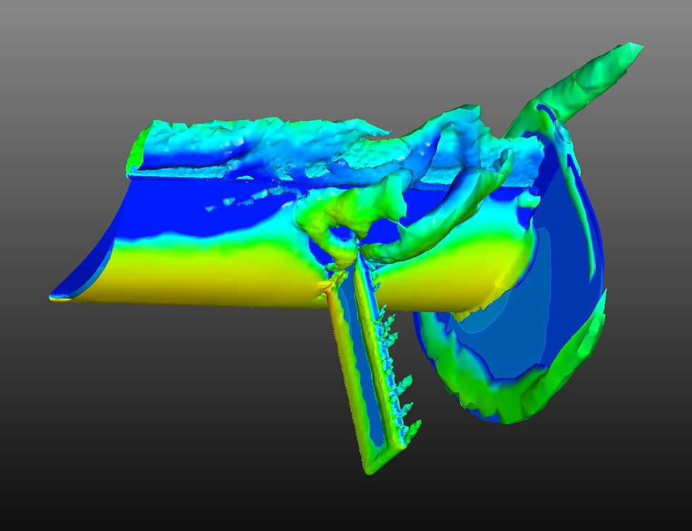
Figure 21: Wall shear stress and vortex plots highlighting highly turbulent flow aft of the wing pylon with the lower surface mount.

3D streamlines help trace the path of air particles passing the pylons; highlighting the chaotic path of air with the lower surface mounting configuration. 

Figure 22: 3D streamlines tracing the flow of air particles past the wing pylons in the HP (left) and LP (right) configurations.

The additional drag can be explained by the larger pylon surface area presenting when routing from the 'boot' surface to the HP aerofoil surface. This does not always have to be the case - as with prototype or formula cars for example which can mount from the engine cover to mitigate this effect.

I prefer the HP configuration here.

Feel the Power

To finish off, I thought it interesting to plot our final wing’s performance over a range of speeds: 50, 100, 150 and 200mph.

Table 8: The performance of our final aerofoil at a range of speeds.

At 200mph, that’s a lot of drag, Increasing by the square of speed!

Now in terms of engine power, let’s see how much you need to pull just the rear wing through the air.

Table 9: Power required to pull the wing through the air at various speeds.

Not an insignificant number by any means, especially when you work the mechanical losses of the drivetrain into the equation!

Conclusions

We haven’t been working with a -L/D target in mind throughout this study; in a practical scenario we’d have probably traded off a little too much efficiency in the pursuit for downforce, but we’ve certainly figured out the flow mechanics of a wing, which would make the design of a higher efficiency variant a pretty straight forward task.

Mission accomplished - I, and hopefully you can now answer the question “What makes an effective rear wing?”.

We have understood the aerodynamic considerations of aerofoils and how to set about getting the most out of a certain chord and span - within the application of a GT style racecar at least.

Of course there are always ‘buts’ - in the objective to try and understand the various positives and negatives of each aerofoil profile and configuration, we worked in discrete steps; +/- 5° on AoA, +/- whole tenths on the variation of aerofoil parameters. This can logically bring you to wonder what’s the gaps in the data might tell you. This could have been addressed by running an iterative script to work in much smaller steps and present us with the ‘perfect’ wing, but the flow mechanisms at work wouldn’t have been so distinguishable from one another and we wouldn’t have learnt as much.

I was hesitant in selecting the ‘optimal’ wing profile following the DoE - judgement could identify the best characteristics from the 3 variables, but perhaps when combined together they interact to the detriment of performance? It would also have been reassuring to correlate the CFD to a physical wing model and get some measured data in efforts to verify the simulation results.

The list goes on, ultimately you have to draw a line to the depth of any study or it can quickly snowball and defeat the original intention.

Hope you’ve enjoyed the process anyway, there will be a follow up article soon looking at answering another question I have - what are the effects of rain, humidity and temperature on aerodynamic performance?

I welcome any discussion, questions or consultation requests you might have after reading this.